Theory
This section describes the theory behind the various Bayesian model fitting schemes in AssayTools.
Bayesian analysis
AssayTools uses Bayesian inference to infer unknown parameters (such as ligand binding free energies) from experimental spectroscopic data. It does this to allow the complete uncertainty—in the form of the joint distribution of all unknown parameters—to be rigorously characterized. The most common way to summarize these results is generally to extract confidence intervals of individual parameters, but much more sophisticated analyses—such as examining the correlation between parameters—are also possible.
The Bayesian analysis scheme is intended to be modular, and the user can select whether certain effects (such as inner filter effects) are incorporated into the model. Below, we describe the components of the model. If an effect that carries unknown nuisance parameters (such as extinction coefficients for inner filter effects), these nuisance parameters carry additional prior terms along with them and are inferred as part of the inference procedure.
Unknown parameters
For convenience, we define the unknown parameters in the model for reference:
- the true total ligand concentration
 in the well (including all species involving the ligand)
 - the true receptor concentration
 (including all species involving the receptor)
Data
For each experiment, the data is given by a set of observations for each well. Each well is associated with some properties:
- the volume
 of sample in the well (mostly buffer)
 - a total concentration
![[R]_T](_images/math/0739690643bd13a973e4aefa0c75415ecb26667a.png) of receptor added to the well
of receptor added to the well - a total concentration
![[L]_T](_images/math/99d2463950f057f43a079460561a1deedbfcfc57.png) of ligand added to the well (or potentially multiple ligands)
of ligand added to the well (or potentially multiple ligands) - the well area
 with the assumption that the well is cylindrical (allowing the path length
  to be computed)
and one or more experimental measurements:
- a top fluorescence measurement (returning toward the incident excitation light)

- a bottom fluorescence measurement (proceeding in the same direction as the incident excitation light)

- an absorbance measurement
Priors
Each unknown parameter in the model is assigned a prior distribution that reflects the state of knowledge we have of its value before including the effects of the observed data.
Concentrations
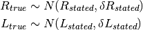
While we design the experiment to dispense the intended amount of protein and ligand into each well, the true amount dispensed into the well will vary due to random pipetting error.
The true concentrations of protein and ligand in each well are therefore unknown.
Because we propagate the pipetting error along with the intended concentrations, we have the intended (“stated”) protein concentration  and its standard error
  as input.
Similarly, the stated ligand concentration
as input.
Similarly, the stated ligand concentration  and its error
  are also known.
If we assume the dispensing process is free of bias, the simplest distribution that fits the stated concentration and its standard deviation without making additional assumptions is a Gaussian.
We assign these true concentrations for the receptor and ligand a prior distribution.
If concentration_priors is set to gaussian, this is precisely what is used
This is expressed in the pymc model as
Ptrue = pymc.Normal('Ptrue', mu=Pstated, tau=dPstated**(-2)) # M
Ltrue = pymc.Normal('Ltrue', mu=Lstated, tau=dLstated**(-2)) # M
Note
pymc uses the precision  instead of the variance
  as a parameter of the normal distribution.
Gaussian priors have the unfortunate drawback that there is a small but nonzero probability that these concentrations would be negative, leading to nonsensical (unphysical) concentrations.
To avoid this, we generally use a lognormal distribution (selected by concentration_priors='lognormal').
Note
The parameters of a lognormal distribution differ from those of a normal distribution by the relationship described here. The parameters above ensure that the mean concentration is the stated concentration and the standard deviation is its experimental uncertainty. The relationship between the mean and variance of the normal distribution  and the parameters for the lognormal distribution is given by:
![\mu_{LN} = \ln \frac{\mu_N^2}{\sqrt{\mu_N^2 + \sigma_N^2}} \:\:;\:\: \sigma^2_{LN} = \ln \left[ 1 + \left( \frac{\sigma_N}{\mu_N}\right)^2 \right] \:\:;\:\: \tau_{LN} = \ln \left[ 1 + \left( \frac{\sigma_N}{\mu_N}\right)^2 \right]^{-1}](_images/math/6f07a536e8e07ca53c27f220e1de06ca4c91e491.png)
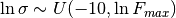
Binding free energy
The ligand binding free energy  is unknown, and presumed to either be unknown over a large uniform range with the
 uniform prior

where we by default take 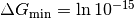 (femtomolar affinity) and Delta G_mathrm{max} = 0 (molar affinity), where is in units of thermal energy
  .
.
This is expressed in the pymc model as
# binding free energy (kT), uniform over huge range
DeltaG = pymc.Uniform('DeltaG', lower=DG_min, upper=DG_max)
This uniform prior has the drawback that affinities near the extreme measurable ranges are simply unknown with equal likelihood out to absurd extreme values.
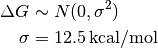
We can attenuate the posterior probabilities at extreme affinities by using a prior inspired by the range of data recorded in ChEMBL via the chembl prior, with a Gaussian form
This is expressed in the pymc model as
# binding free energy (kT), using a Gaussian prior inspired by ChEMBL
DeltaG = pymc.Normal('DeltaG', mu=0, tau=1./(12.5**2))
Modular components of the Bayesian model
We now discuss the various modular components of the Bayesian inference scheme.
These components generally involve models of observed spectroscopic value that are computed from concentrations of the various components ![[X_i]](_images/math/da36231822672036e8ae46364cdbe98cc5fc71ae.png) which represent, for example, free receptor
which represent, for example, free receptor  , complexed receptor
  , or free ligand
  .
These concentrations are computed from the current samples of true total concentrations and binding affinities using one of the specified binding models described below.
.
These concentrations are computed from the current samples of true total concentrations and binding affinities using one of the specified binding models described below.
Fluorescence
Fluorescence model.
Fluorescence can be measured from either the top, bottom, or both.
The true fluorescence depends on the concentration of each species  :
:
![F_\mathrm{top} = I_{ex} \left[ \sum_{i} q_i(ex,em) [X_i] + l F_\mathrm{buffer} + F_\mathrm{plate} \right]
F_\mathrm{bottom} = G_\mathrm{bottom} \cdot I_{ex} \left[ \sum_{i} q_i(ex,em) [X_i] + l F_\mathrm{buffer} + F_\mathrm{plate} \right]](_images/math/02834d5a8b6e36097fe2b0f0a0c1145696ce3622.png)
Here,  is the incident excitation intensity,
  are the quantum efficiencies of each species at the excitation/emission wavelengths,
  is a buffer fluorescence per unit path length, and
  is the background fluorescence of the plate.
Notably, without inner filter effects, the only factor that causes differences between top and bottom fluorescence is the gain factor G_mathrm{bottom} that captures a potential difference in detector gains between the top and bottom detectors.
is the background fluorescence of the plate.
Notably, without inner filter effects, the only factor that causes differences between top and bottom fluorescence is the gain factor G_mathrm{bottom} that captures a potential difference in detector gains between the top and bottom detectors.
Observed fluorescence.
The observed fluorescence  and
and  will differ from the true fluorescence due to detector noise.
Because the observed fluorescence is reported as the mean of a number of detector measurements from independent flashes of the Xenon lamp, detector error will be well described by a normal distribution:
will differ from the true fluorescence due to detector noise.
Because the observed fluorescence is reported as the mean of a number of detector measurements from independent flashes of the Xenon lamp, detector error will be well described by a normal distribution:
The measurement errors  and
and  are assigned Jeffreys priors, which are uniform in
By default, the same detector error  is used for both top and bottom detectors, but separate errors can be used if
 link_top_and_bottom_sigma = False.
While the detector error is inferred separately for each experiment since the detector gain may differ from experiment. If multiple datasets using the same instrument configuration and detector gain are inferred together—such as the inclusion of calibration experiments with controls—this will help improve the detector error estimate.
Quantum efficiencies.
Since the quantum efficiencies of each species are unknown, they are inferred as nuisance parameters as part of the Bayesian inference process.
We therefore assign a uniform (informationless) priors to these, though we use the product 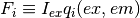 for convenience since and the scaling factor to convert observed fluorescence into reported arbitrary fluorescence units is unknown:
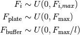
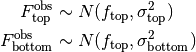
For efficiency, we compute the maximum allowed values based on an upper limit of these quantities from the observed data.
We also make efficient initial guesses for these quantities, which assume that:
- assumes the minimum fluorescence signal is explained by only buffer fluorescence
- assumes the minimum fluorescence signal is explained by only plate fluorescence
 assumes the maximum fluorescence signal increase above background is explained by the free ligand fluorescence
 assumes the receptor fluorescence is zero
 assumes that the maximum fluorescence signal increase above background is explained by complex fluorescence with 100% complex formation
These assumptions can of course be violated once the sampler starts to infer these quantities.
In the pymc model, these priors are implemented via
model['F_PL'] = pymc.Uniform('F_PL', lower=0.0, upper=2*Fmax/min(Pstated.max(),Lstated.max()), value=F_PL_guess)
model['F_P'] = pymc.Uniform('F_P', lower=0.0, upper=2*(Fmax/Pstated).max(), value=F_P_guess)
model['F_L'] = pymc.Uniform('F_L', lower=0.0, upper=2*(Fmax/Lstated).max(), value=F_L_guess)
model['F_plate'] = pymc.Uniform('F_plate', lower=0.0, upper=Fmax, value=F_plate_guess)
model['F_buffer'] = pymc.Uniform('F_buffer', lower=0.0, upper=Fmax/path_length, value=F_buffer_guess)
If an estimate of is known from a prior experiment, this value and its standard error can be specified via a lognormal distribution
model['F_PL'] = pymc.Lognormal('F_PL', mu=np.log(F_PL**2 / np.sqrt(dF_PL**2 + F_PL**2)), tau=np.sqrt(np.log(1.0 + (dF_PL/F_PL)**2))**(-2))
Top/bottom detector gain.
The bottom detector relative gain factor is assigned a uniform prior over the log gain:
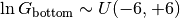
which is implemented in the pymc model as
model['log_gain_bottom'] = pymc.Uniform('log_gain_bottom', lower=-6.0, upper=6.0, value=log_gain_guess)
Absorbance
Absorbance model.
The absorbance is determined by the the extinction coefficient of each component (R, L, RL for simple two-component binding) at the illumination wavelength, as well as any intrinsic absorbance of the plate at that wavelength.
![A &= 1 - e^{-\epsilon \cdot l \cdot [L]}](_images/math/52aaf31633a21e93dd93bd8569554761ef420560.png)
where  is the extinction coefficient of the species (e.g. free ligand ) at the illumination wavelength (excitation or emission), is the path length, and
  is the concentration of the species.
Note
You may be more familiar with the linearized form of Beer’s law ( ). It’s easy to see that this comes from a Taylor expansion of the above equation, truncated to first order:
 ![1 - e^{-\epsilon l c} \approx 1 - \left[ 1 - \epsilon l c + \mathcal{O}(\epsilon l c)^2) \right] \approx \epsilon l c](_images/math/344bb4b27521f59272cf245b85c5308fd46c4da5.png) . We use the equation above instead because it is much more accurate for larger absorbance values.
. We use the equation above instead because it is much more accurate for larger absorbance values.
The plate absorbance is a nuisance parameter that is assigned a uniform informationless prior:
Currently, AssayTools supports absorbance measurements made at either (or both) the excitation and emission wavelengths.
Absorbance measurements performed at the excitation wavelength help constrain the extinction coefficient for primary inner filter effects, while absorbance measurements at the emission wavelength help constrain the extinction coefficients for secondary inner filter effects.
Note that even if plates that are not highly transparent in the excitation or emission wavelengths are used, this still provides useful information—this effect is corrected for by inferring the plate absorbance  at the appropriate wavelengths.
Note
Currently, AssayTools only models absorbance for the ligand, using data from wells in which only ligand in buffer is present. In the future, we intend to extend this to support absorbance of all components.
Observed absorbance.
As the detector averages many measurements from multiple flashes of a Xenon lamp for the reported absorbance  , the observed measurement can be modeled with a normal distribution
The detector error  is assigned Jeffreys priors, which are uniform in
Note
It is critical that if multiple datasets are inferred jointly, they all be from the same plate type.
Inner filter effects
Primary inner filter effect.
At high ligand concentrations, if the ligand has significant absorbance at the excitation wavelength, the amount of light reaching the bottom of the well is less than the light reaching the top of the well. This is called the primary inner filter effect, and has the net effect of attenuating the observed absorbance and fluorescence.
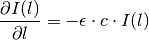
To see where this effect comes from, consider the permeation of light through a liquid with molar concentration , and extinction coefficient .
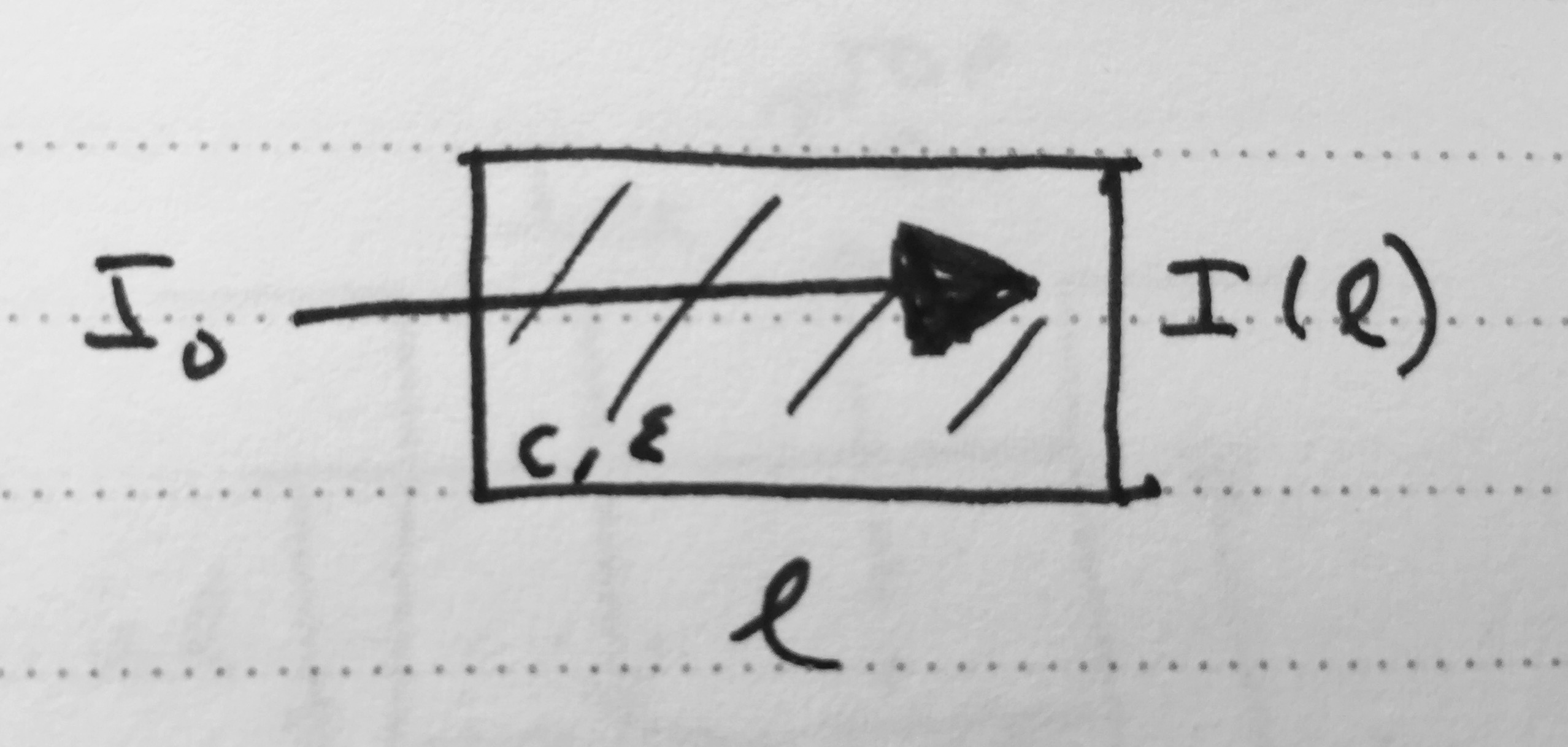
Attenuation of light passing through a liquid containing absorbing species.
A slice of width  at depth will absorb some of the incoming light intensity
  :
:

If we shrink down to an infinitesimal slice, this gives us a differential equation for the intensity at depth :
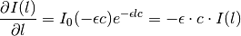
It’s easy to see that the solution to this differential equation is given by
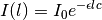
since this satisfies the differential equation:
If only the primary inner filter effect is used, both top and bottom fluorescence are attenuated by a factor that can be computed by integrating the attenuation of incident light over the whole liquid path length:
![\mathrm{IF}_\mathrm{top/bottom} = \int_0^1 dx e^{-\epsilon_{ex} \cdot x l \cdot c} = \left[ \frac{e^{-\epsilon_{ex} \cdot x l \cdot c}}{-\epsilon_{ex} \cdot l \cdot c} \right]_0^1 = \frac{1 - e^{-\epsilon_{ex} \cdot l \cdot c}}{\epsilon_{ex} \cdot l \cdot c}](_images/math/c4827aa961e8016aae3fda0c135febeb95fb67f8.png)
Note
When  , numerical underflow of the exponential becomes a problem. To avoid negative attenuation factors, a fourth-order Taylor series approximation of the exponential is used in computing the attenuation factor if
  .
.
Note
Currently, inner filter effects are only computed for the free ligand, but we plan to extend this to include a sum over the effects from all species.
Secondary inner filter effect.
Similarly, the secondary inner filter effect is caused by significant absorbance at the emission wavelength. When both effects are combined, the net attenuation effect depends on the geometry of excitation and detection:

Geometry and light intensities used for inner filter effect corrections.
, transmitted light  , and emitted fluorescent light toward the top
  and bottom
  detectors.
The distance from the top liquid interface is expressed in terms of the dimensionless
detectors.
The distance from the top liquid interface is expressed in terms of the dimensionless ![x \in [0,1]](_images/math/3ee01caaddd426cf9eb9824181b5e254331ca9a2.png) and the path length
and the path length  , with liquid volume and well area .
Consider the shaded slice at depth  depicted in the figure.
The excitation light reaching this layer has intensity
depicted in the figure.
The excitation light reaching this layer has intensity
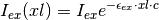
where is the concentration of the species with extinction coefficient  (where we are only considering the effects from the ligand species at this point, since its concentration can be high).
The secondary inner filter effect, because it considers absorbance at a different wavelength from the incident light, does not attenuate the absorbance.
If both primary and secondary inner filter effects are utilized, fluorescence is attenuated by a factor that depends on the detection geometry.
For top fluorescence, this is given by

For bottom fluorescence measurements, the path taken to the detector is different from the incident path length, so the attenuation factor is given by
![\mathrm{IF}_\mathrm{bottom} = \int_0^1 dx \, e^{-\epsilon_{ex} \cdot xl \cdot c} \, e^{-\epsilon_{em} \cdot (1-x)l \cdot c} = e^{-\epsilon_{em} l c} \int_0^1 dx \, e^{-(\epsilon_{ex} - \epsilon_{em}) \cdot xl \cdot c} = e^{-\epsilon_{em} l c} \left[\frac{1 - e^{-(\epsilon_{ex} - \epsilon_{em}) l c}}{(\epsilon_{ex} - \epsilon_{em}) l c} \right]](_images/math/e0e14ab2e28ab71445dce2af679b7512f4db0416.png)
Note
Just as with the primary inner filter effect, when  , numerical underflow of the exponential becomes a problem. To avoid negative attenuation factors, a fourth-order Taylor series approximation of the exponential is used in computing the attenuation factor if
  .
.
Extinction coefficients
Extinction coefficients at excitation (and possibly emission) wavelengths are needed if either absorbance measurements are made or inner filter effects are used. These can either be measured separately and provided by the user or inferred directly as nuisance parameters.
Measured extinction coefficients.
If the extinction coefficients have been measured, we have a measurement and corresponding standard error  available.
Because extinction coefficients must be positive, we use a lognormal distirbution to model the true extinction coefficients about the measured value
available.
Because extinction coefficients must be positive, we use a lognormal distirbution to model the true extinction coefficients about the measured value
![\epsilon \sim \mathrm{LN}(\mu, \tau) \:\:\mathrm{where}\:\: \mu = \ln \frac{\epsilon^2}{\sqrt{\epsilon^2 + \delta^2 \epsilon}} \:\:,\:\: \tau = \ln \left[ 1 + \left( \frac{\delta \epsilon}{\epsilon}\right)^2 \right]^{-1}](_images/math/855bc016411824e57e8d024cb9f682c87b8e5e9e.png)
Inferred extinction coefficients.
If the extinction coefficients have not been measured, they are inferred as nuisance parameters, with priors assigned from a uniform distribution with a large maximum and an initial guess based on the extinction coefficient of bosutinib at 280 nm
model['epsilon_ex'] = pymc.Uniform('epsilon_ex', lower=0.0, upper=1000e3, value=70000.0) # 1/M/cm
model['epsilon_em'] = pymc.Uniform('epsilon_em', lower=0.0, upper=1000e3, value=0.0) # 1/M/cm
Binding models
AssayTools has a variety of binding models implemented.
Though the user must currently specify the model to be fit to the data, we plan to include the ability to automatically select the most appropriate binding model automatically using reversible-jump Monte Carlo (RJMC), which also permits Bayesian hypothesis testing.
All binding models are subclasses of the BindingModel abstract base class, and users can implement their own binding models as subclasses.
Two-component binding model
A two-component binding model is implemented in assaytools.bindingmodels.TwoComponentBinding.
When it is known that receptor R associates with ligand L in a 1:1 fashion, we can write the dissociation constant  in terms of the equilibrium concentrations of each species:
![K_d = \frac{[R][L]}{[RL]}](_images/math/afcb058a78fb71bcc0c96cda43c76e6d106158a5.png)
Incorporating conservation of mass constraints
![[R]_T &= [R] + [RL] \\
[L]_T &= [L] + [RL]](_images/math/607c873501c4e3fb46ba817bd08f3dacc4091249.png)
we can eliminate the unknown concentrations of free receptor ![[R]](_images/math/09ff738d6a28ea9eb228fc2d91ee23d60de09af7.png) and free ligand
and free ligand ![[L]](_images/math/e2f42dbc3cff1602eac7aaa1fe8f92b07bc7ac48.png) to obtain an expression for the complex concentration
to obtain an expression for the complex concentration ![[RL]](_images/math/6b737aa502b87c53f7c691d37a4ba6ee62d4c84e.png) in terms of fixed quantities (dissociation constant and total concentrations and ):
in terms of fixed quantities (dissociation constant and total concentrations and ):
![K_d = \frac{([R]_T - [RL]) ([L]_T - [RL])}{[RL]}
[RL] K_d = ([R]_T - [RL]) ([L]_T - [RL])
0 = [RL]^2 - ([R]_T + [L]_T + K_d) [RL] + [R]_T [L]_T](_images/math/f5bcc3afb9c1d167fa1306ce9ad474da220a0854.png)
This quadratic equation has closed-form solution, with only one branch of the solution where we require
![0 < [RL] < \min([R]_T, [L]_t)](_images/math/7027b3c6c82c80aacdf5a09cbf38d6f5aa63af15.png)
which gives
![K_d = \frac{1}{2} \left[ ([R]_T + [L]_T + K_d) - \sqrt{([R]_T + [L]_T + K_d)^2 - 4 [R]_T [L]_T} \right]](_images/math/963ca89c8fe2b2c6697d2474a38bf7368f2608ea.png)
Note that this form is not always numerically stable since , , and may differ by orders of magnitude, leading to slightly negative numbers inside the square-root.
AssayTools uses the logarithms of these quantities instead, and guards against negative values inside the square root.
Competitive binding model
When working with N ligands  that bind a single receptor , we utilize a competitive binding model implemented in
 assaytools.bindingmodels.CompetitiveBindingModel.
Here, the dissociation constants  are defined as
![K_n = \frac{[R][L_n]}{[RL_n]}](_images/math/095639699aeaa15919b697c5120f486613c0348e.png)
with corresponding conservation of mass constraints
![[R]_T &= [R] + \sum_{n=1}^N [RL_n] \\
[L_n]_T &= [L_n] + [RL_n], n = 1,\ldots, N](_images/math/9a65e4ca2583a4b71d50be41c3f0c1dbd740f95b.png)
The solution must also satisfy some constraints:
![0 \le [RL_n] \le \min([L_n], [R]_T) \:\:,\:\: n = 1,\ldots,N
\sum_{n=1}^N [RL_n] \le [R]_T](_images/math/27fa9aad063dcc06bdb80920dbe885a0fe1d7592.png)
We can rearrange these expressions to give
![[R][L_n] - [RL_n] K_n = 0 \:\:,\:\: n = 1, \ldots, N](_images/math/c92cd3c9816019b5af7f7378bc714b1fe72b83f9.png)
and eliminate ![[RL_n]](_images/math/c439f8f685f88337f304825be2b97411d8be8203.png) and to give
and to give
![\left( [R]_T - \sum_{n=1}^N [RL_n] \right) \cdot ([L_n]_T - [RL_n]) - [RL_n] K_n = 0 \:\:,\:\: n = 1, \ldots, N](_images/math/0223aaacf8e0884119154acc6a0dd24e6aac661b.png)
This leads to a coupled series of equations that cannot easily be solved in closed form, but are straightforward to solve numerically using the solver scipy.optimize.fsolve(), starting from an initial guess that ensures the constraints remain satisfied.
General binding model
A more general binding model is available in assaytools.bindingmodels.GeneralBindingModel.
A general series of  equilibrium reactions involving the interconversion of
  components
  , which may represent individual species or complexes, and have the form
![K_n = \prod_{j=1}^K [X_j]^{s_{nj}} \:\: , \:\: n = 1,\ldots,N](_images/math/034b44b393f1787bf7a8d7c29a611a437cb9f7a3.png)
with corresponding conservation of mass constraints
![\sum_{j=1}^K c_{mj} [X_j] = q_m \:\: , \:\: m = 1,\ldots,M](_images/math/66cea46ab340e56602b15deca2612118358b2bd2.png)
This problem can be specified in terms of
- an
 equilibrium constant vector
- an
 stoichiometry matrix
- an
 mass conservation matrix
- an
 -vector
  of total concentrations across all species
For example, for a simple binding reaction 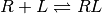 , the species are
  , and we have
![K &= [K_d] \\
S &= \begin{bmatrix}
+1 & +1 & -1
\end{bmatrix} \\
C &= \begin{bmatrix}
+1 & 0 & +1 \\
0 & +1 & 0
\end{bmatrix} \\
Q &= \begin{bmatrix}
[R]_\mathrm{tot} \\
[L]_\mathrm{tot}
\end{bmatrix}](_images/math/25c11a4716dc7947638eab451be6157b846dddae.png)
A competitive binding reaction and 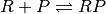 with species
  , we have
![K &= \begin{bmatrix}
K_1 \\
K_2 \\
\end{bmatrix} \\
S &= \begin{bmatrix}
+1 & +1 & 0 & -1 & 0 \\
+1 & 0 & +1 & 0 & -1 \\
\end{bmatrix} \\
C &= \begin{bmatrix}
+1 & 0 & 0 & +1 & +1 \\
0 & +1 & 0 & +1 & 0 \\
0 & 0 & + & 0 & +1 \\
\end{bmatrix} \\
Q &= \begin{bmatrix}
[R]_\mathrm{tot} \\
[L]_\mathrm{tot} \\
[P]_\mathrm{tot}
\end{bmatrix}](_images/math/a78585ab8397cd23da16ee7837236757b3d08092.png)
Because the equilibrium constants and concentrations ![[X_j]](_images/math/4ccf4d1e413d56ee6ee1cfd184b0cdf5f88f388b.png) must be positive but can range over many orders of magnitude, we represent these quantities by their logarithms, resulting in the equations
must be positive but can range over many orders of magnitude, we represent these quantities by their logarithms, resulting in the equations
![0 &= - \log K_n + \sum_{j=1}^K s_{nj} \log [X_j] \:\: , \:\: n = 1,\ldots,N \\
0 &= - \log q_m + \log \sum_{j, c_{mj} > 0} e^{\log c_{mj} + \log [X_j]} \:\: , \:\: m = 1,\ldots,M \\](_images/math/79fc424d9180d20eb424e3cb55cf0576febbe67d.png)
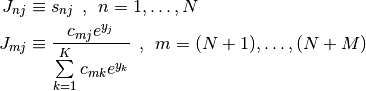
The equilibrium concentrations is found as the solution to this set of equations using ![y_j \equiv \log [X_j]](_images/math/0fa37702c26ac6e9247979ea4aa630fce671fa46.png) , solved by the numerical root-finding function
, solved by the numerical root-finding function scipy.optimize.root() using the vector-valued function  and its Jacobian
  :
:
![f_n(x) &\equiv - \log K_n + \sum_{j=1}^K s_{nj} \log [X_j] \:\: , \:\: n = 1,\ldots,N \\
f_m(x) &\equiv - \log q_m + \log \sum_{j, c_{mj} > 0} e^{\log c_{mj} + \log [X_j]} \:\: , \:\: m = (N+1),\ldots,(N+M)](_images/math/ac7acd5b71c12ed8b564ba97c6ed69fa8977054a.png)
where the  operation can be computed in a numerically stable manner using the
 scipy.misc.logsumexp() function.
The Jacobian is given by
where the scipy.misc.logsumexp() function is once again used to compute rows  in a numerically stable manner.